I previously wrote about how Mastra orchestrates agents and handles guardrails. In the sequence of exploring Mastra’s RAG support, I took a detour: I wanted to understand how vector databases work under the hood instead of treating them as a black box. That detour turned into a deep dive into pgvector, HNSW indexing, embedding models, tokenization, chunking strategies etc.

I usually keep my blogs as a scratchpad. When an area interests me, I write down what I learn here in journal form. Vector databases and RAG are a good fit for that. The information on them is fragmented across papers, library docs, and blog posts. This post gathers the layers in one place so I can reference them together.

---

This is not a deep dive into any single component. It is an exploration of how tokenizers, embeddings, indexes, and search all connect — and how you can wire them together to build something like a semantic search engine. Let’s carry one paragraph through the whole pipeline so we can see the transformation at each stage:

The cat sat on the mat and watched the birds fly south for winter. Every autumn, the swallows left the garden in a loose flock and flew toward the coast, where the marshlands held enough insects and seeds to carry them through the cold months. The cat knew the pattern. It had watched the same migration for seven seasons from its mat by the kitchen door, and each year the birds departed a few days earlier. When the last swallow vanished past the old oak, the garden fell quiet and the cat went inside.

By the end of this post, we will know exactly how this paragraph becomes a set of vectors.

---

Before we dive in: this stack has distinct layers. The abbreviations look like they belong together, which is where the confusion starts. A vector database has two halves. The first half is encoding: turning text into searchable vectors. It has three categories of tools, and the names you see online are examples of each. The lists below are not exhaustive — each category has many more implementations. These are the popular ones you will actually meet in the wild:

• Tokenization algorithms — split raw text into token IDs. Popular examples: BPE (Byte Pair Encoding), WordPiece, Unigram.
• Embedding models — convert token IDs into vectors. Popular examples: Word2Vec, BERT (Bidirectional Encoder Representations from Transformers), MiniLM.
• Indexing algorithms — organize vectors for fast search. Popular examples: IVFFlat, HNSW (Hierarchical Navigable Small World).

These three categories are not competing alternatives. They operate at completely different stages:

Category	Popular examples	What it does
Tokenization algorithm	BPE, WordPiece, Unigram	splitting text into token IDs
Embedding model	Word2Vec, BERT, MiniLM	converting token IDs into vectors
Indexing algorithm	IVFFlat, HNSW	organizing vectors for fast search

Think of it as a factory line: BPE cuts raw text into pieces. BERT reads those pieces and produces vectors. An indexing algorithm like HNSW files those vectors so you can find them later. Each stage feeds the next.

---

Table of Contents

1. Tokenization — splitting text into tokens
2. From Tokens to Vectors — Word2Vec, BERT, sentence embeddings, and the levels by use case

Continue to Part 2: Dimensions, Chunking, and Similarity for what dimensions capture, chunking strategies, and the distance functions that rank results.

---

1. Tokenization

Every language model starts with the same problem: text is a string of characters, but machines need numbers.

Tokenization splits raw text into chunks called tokens. A token can be a word, a subword, or a single character. The model never sees letters. It sees token IDs.

The Three Main Approaches

Virtually every LLM and embedding model in production today uses one of three subword tokenizers: BPE, WordPiece, or Unigram. How each one builds its vocabulary and merges tokens is a research topic on its own. The HuggingFace tokenizer docs explain the mechanics in detail, so I am not going to repeat them here. For this post the tokenizer is a tool I call, not a system I build. What matters is which models use which:

Approach	Used by
BPE	GPT-4o (tiktoken), GPT-2, RoBERTa
WordPiece	BERT, DistilBERT, MiniLM (30k vocabulary)
Unigram	LLaMA, T5, ALBERT via SentencePiece (32k vocabulary)

tiktoken, the tokenizer behind OpenAI’s models, is BPE with a different vocabulary file per model. Each row links to the loader in tiktoken’s repo for that encoding:

Encoding	Vocab	Used by	Vocab file
cl100k_base	100K	GPT-4, GPT-3.5-turbo, text-embedding-3	tiktoken_ext/openai_public.py L75–93
o200k_base	200K	GPT-4o	tiktoken_ext/openai_public.py L95–122
r50k_base	50K	GPT-3, Codex, text-davinci-003, ada-002	tiktoken_ext/openai_public.py L33–45
p50k_base	50K	code-cushman-001	tiktoken_ext/openai_public.py L47–59

Tokenization Matters for Retrieval

Context windows count tokens, not words. A 512-token limit for an embedding model means 350-400 English words. The exact count depends on the tokenizer the embedding model uses, and the same text costs different amounts across models.

Our example paragraph makes it concrete: the Xenova/all-MiniLM-L6-v2 tokenizer (the one the app and the visualizer use) converts the 94 words above into 106 tokens — the paragraph plus [CLS] and [SEP]. The next section shows the code that produces that number, and the visualizer lets you watch it happen.

Counts drift between tokenizer versions, so profile your exact model. Always count tokens, not words.

Our Example Tokenized

Here is the full example paragraph with HuggingFace’s tokenizer, a WordPiece tokenizer sharing BERT’s vocabulary. The paragraph runs to 106 IDs including [CLS] and [SEP]:

packages/shared/src/index.ts L3

import { AutoTokenizer } from "@huggingface/transformers";

const tokenizer = await AutoTokenizer.from_pretrained("Xenova/all-MiniLM-L6-v2");

const text =
  "The cat sat on the mat and watched the birds fly south for winter. " +
  "Every autumn, the swallows left the garden in a loose flock and flew " +
  "toward the coast, where the marshlands held enough insects and seeds " +
  "to carry them through the cold months. The cat knew the pattern. It " +
  "had watched the same migration for seven seasons from its mat by the " +
  "kitchen door, and each year the birds departed a few days earlier. " +
  "When the last swallow vanished past the old oak, the garden fell " +
  "quiet and the cat went inside.";
const { input_ids } = await tokenizer(text);

console.log(Array.from(input_ids.data).length);
// 106 (includes [CLS] at 101, [SEP] at 102)

The visualizer below is that logic in action. It loads the same Xenova/all-MiniLM-L6-v2 tokenizer from HuggingFace, defaults to the example paragraph, and colors each token by its ID.

You can edit the text above in real time and watch how the tokenizer splits it into tokens. Two details need explaining before anything else.

The tokens with a golden ring are [CLS] and [SEP] — special tokens that the tokenizer injects automatically, covered in detail below. They are the only tokens in the output that are not words from the paragraph.

Why This Model?

MiniLM is Microsoft’s compressed BERT (Wang et al., 2020). all-MiniLM-L6-v2 keeps BERT’s WordPiece tokenizer and its 30,522-token vocabulary, which matches BERT’s own vocab exactly, then shrinks the network: 6 layers instead of 12, and 384 dimensions instead of 768. Same tokens as BERT, a fraction of the weights, small enough to run in a browser tab.

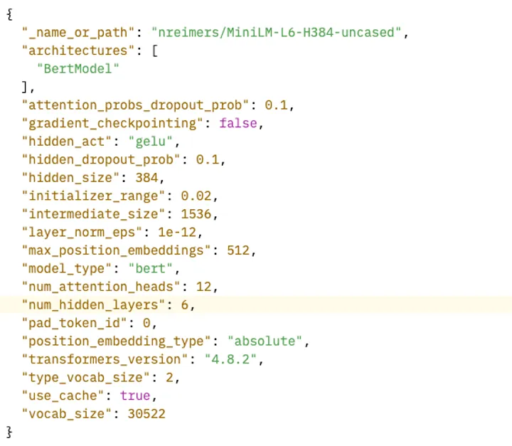
These posts use it because the whole stack runs in the browser through transformers.js straight from HuggingFace. No API key, no server, and the model files cache after the first load. The visualizer below loads that same tokenizer and colors each token by its ID.

Everything else in the output is words from the paragraph, and it helps to anchor on one sentence. Take the sentence in the middle:

". The cat knew the pattern."

It appears in the token stream as

".the cat knew the pattern ."

The capitalized “The” is not a special token and is not skipped. It is lowercased and lands on the same ID as every other “the” in the paragraph, 1996, which is why all of them share one color in the visualizer. The model is uncased.

Both facts are in the same tokenizer_config.json: "cls_token": "[CLS]", "sep_token": "[SEP]", and "do_lower_case": true.

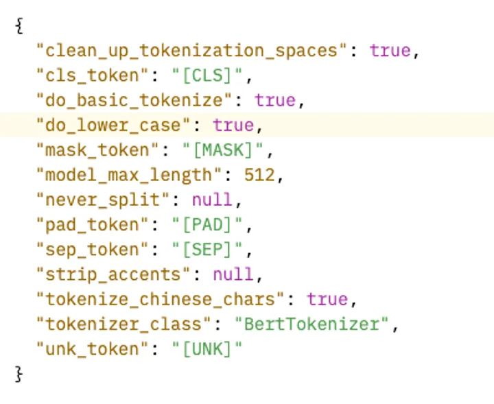
Now look at the words themselves: no token carries a leading space. “the” appears as “the”, not ” the”. That is not a display choice — it follows from the vocabulary the tokenizer loads. The same tokenizer_config.json declares "tokenizer_class": "BertTokenizer", which reads a vocab.txt with exactly 30,522 lines (the vocab_size from the config above):

$ wc -l vocab.txt
30522 vocab.txt

$ grep -c "^ $" vocab.txt
0

$ grep -c "^ " vocab.txt
0

There is no token for a bare space, and no token that starts with one. Every entry is a word or a word-piece, and pieces that continue a word are marked with a ”##” prefix. A ## token can never begin a word; it only completes the token before it. That is the philosophy of BERT-style tokenizers: instead of storing every rare word as its own entry, the vocabulary keeps common fragments like ##ing, ##ed, and ##lands and assembles any word from a few pieces. Since spaces cannot be encoded, they are dropped and the following word starts clean. That is why “marshlands” has no entry of its own and splits into marsh + ##lands in the token stream above: vocab.txt#L9410 is marsh, vocab.txt#L8654 is ##lands.

The same paragraph, tokenized with tiktoken (the tokenizer GPT-4o uses), shows the opposite convention:

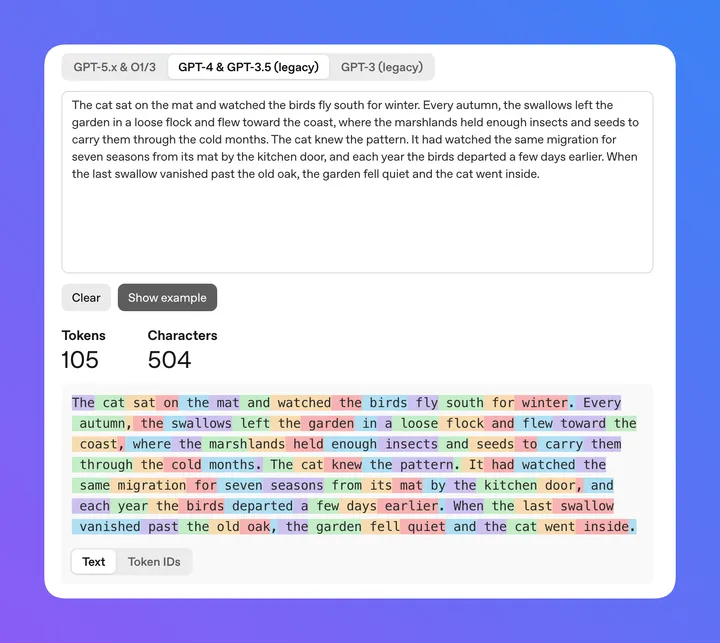
Notice the leading space on ” cat”. tiktoken, like GPT-2, is BPE-based: it treats the space as a character and merges it into the following word, so every word’s first token carries the space that precedes it. Same text, two different token streams, because whitespace handling is a tokenizer decision, not a property of the text.

Special tokens are not part of the original text. The tokenizer injects them before or after the encoded input to signal structure to the model. Each model defines its own set of special tokens in its tokenizer_config.json — this is where the mapping from token ID to semantic meaning lives. The HuggingFace tokenizer docs explain how these are added during encoding:

• [CLS] — A classification token prepended to every input. The BERT paper (Devlin et al., 2019) introduced this convention; the final hidden state at this position is used as the aggregate sequence representation.
• [SEP] — Separates two segments (question/answer, premise/hypothesis) or marks the end of a sequence. Also from the BERT paper.
• [PAD] — Pads all sequences in a batch to the same length. The attention mask tells the model to ignore these positions during self-attention.
• [UNK] — Replaces tokens the vocabulary doesn’t contain. The WordPiece paper (Schuster & Nakajima, 2012) formalized this for subword tokenizers.
• [MASK] — Used during masked language model pre-training (also from BERT).

The model returns these tokens in the same input_ids array as everything else — they go through the same embedding layer, attention layers, and output projections.

---

2. From Tokens to Vectors

In the tokenizer above, you saw text become a list of integers. Those integers are not vectors. This is where beginners get tripped up: the tokenizer and the embedding model are two separate stages. The tokenizer is a deterministic rulebook — it maps text to IDs using a fixed vocabulary (no learning, no math). The embedding model is a neural network that learns to convert those IDs into meaningful vectors.

Token IDs are just integers. An integer cannot capture meaning. The number 1996 (the token ID for “the”) has no semantic relationship to 4937 (“cat”). The embedding layer fixes this.

The Embedding Lookup Table

An embedding layer is a matrix of shape (vocab_size, embedding_dimension). Each row is a trainable vector. The vocabulary size is how many unique tokens the tokenizer knows — every ID in that range has a corresponding row. all-MiniLM-L6-v2, the model running in the tokenizer above, has 30,522 vocabulary entries and an embedding size of 384, so its embedding layer is a 30,522 × 384 matrix. A sequence longer than the model’s context window gets truncated before it reaches the embedding layer. These are two different numbers: GPT-4 has ~100k vocabulary but a 128k context window.

The matrix is one of the model’s trained weight tensors. model.safetensors is the weight file in the sentence-transformers/all-MiniLM-L6-v2 repository on Hugging Face — download it from the repo’s “Files and versions” tab (or wget) and save it next to the script. This script reads the real matrix out of that file and looks up the rows for two tokens:

import { readFileSync } from "node:fs";

// model.safetensors stores weights as a JSON header followed by raw float bytes.
const buffer = readFileSync("model.safetensors");
const headerLength = Number(buffer.readBigUInt64LE(0));
const header = JSON.parse(buffer.subarray(8, 8 + headerLength).toString());

const { shape, data_offsets } = header["embeddings.word_embeddings.weight"];
// shape: [ 30522, 384 ]

const [start, end] = data_offsets;
const bytes = buffer.subarray(start, end);
const weights = new Float32Array(bytes.buffer, bytes.byteOffset, bytes.byteLength / 4);

// The tokenizer above turned "the cat" into the IDs [1996, 4937].
const row = (id) => Array.from(weights.slice(id * 384, id * 384 + 384));
console.log(
  row(1996)
    .slice(0, 8)
    .map((v) => v.toFixed(4)),
); // "the"
console.log(
  row(4937)
    .slice(0, 8)
    .map((v) => v.toFixed(4)),
); // "cat"

The above snippets generates the logs as

[
  '-0.0089', '-0.0102',
  '-0.0419', '0.0178',
  '-0.0057', '0.0192',
  '-0.0153', '-0.0306'
]
[
  '0.0340',  '-0.0389',
  '0.0573',  '-0.0327',
  '-0.1233', '-0.0774',
  '0.0395',  '0.1027'
]

Each row is one vector of 384 numbers. Token ID 1996 picks row 1996, token ID 4937 picks row 4937. That is the whole mechanism — an index into a matrix, nothing more.

Where does the ID-to-word mapping come from? The vocabulary is a plain text file with one entry per ID, so it is directly inspectable: vocab.txt#L1997 is the, and vocab.txt#L4938 is cat. The visualizer above is the same mapping live: hover any token and its ID shows up.

These 384 values start random during training. Training adjusts them so words used in similar contexts move closer together. The matrix above is the trained, final version — the same weights the live model uses for every sentence in this post.

Word2Vec: The First Breakthrough

The lookup table is the static part of the story. Word2Vec (Mikolov et al., 2013) is where training became the point: it learned embeddings by predicting a word from its neighbors, so words that hang around together got similar vectors. Trained vectors even started doing algebra:

vector("king") - vector("man") + vector("woman") ≈ vector("queen")

But it has a hard ceiling: every word gets exactly one vector, forever. “Bank” is the same row by a river or by a vault, and a word never seen during training gets nothing. One word, one meaning, one row — which is exactly what the next idea removes.

BERT and Contextual Embeddings

The fix is to not decide a word’s meaning until it knows its context. The Transformer (Vaswani et al., 2017) introduced self-attention: every token attends to every other token before committing to a vector, so the same token ID produces a different vector in a different sentence. BERT (Devlin et al., 2019) pre-trained that machinery on a large corpus, and all-MiniLM-L6-v2 is a distilled BERT.

Run a nine-token sentence through it and you get nine 384-dimension vectors, one per token, shaped [batch, tokens, dims] = [1, 9, 384]. Context-aware, but still the wrong shape for search: a vector per token, not per text. For how self-attention actually works, the Illustrated Transformer is the best single explanation.

Sentence Embeddings

One vector per token is still the wrong shape for search. You search with a question and a paragraph, not with a word, so the token vectors need to collapse into one vector per text.

The collapse is mean pooling: average the token vectors, ignoring padding, so N vectors become one. Averaging a raw BERT gives a mediocre sentence vector, because BERT never trained for that comparison. Sentence-BERT (Reimers & Gurevych, 2019) fixed it with contrastive training: matching texts get pulled together, non-matching pairs pushed apart, pooling stays a mean, and the result is directly comparable.

all-MiniLM-L6-v2 is exactly that: a distilled BERT, mean-pooled, contrastive-tuned. One call and the whole paragraph becomes 384 numbers:

import { pipeline } from "@huggingface/transformers";

const embedder = await pipeline("feature-extraction", "Xenova/all-MiniLM-L6-v2");

const paragraph =
  "The cat sat on the mat and watched the birds fly south for winter. " +
  "Every autumn, the swallows left the garden in a loose flock and flew " +
  "toward the coast, where the marshlands held enough insects and seeds " +
  "to carry them through the cold months. The cat knew the pattern. It " +
  "had watched the same migration for seven seasons from its mat by the " +
  "kitchen door, and each year the birds departed a few days earlier. " +
  "When the last swallow vanished past the old oak, the garden fell " +
  "quiet and the cat went inside.";

const result = await embedder(paragraph, { pooling: "mean", normalize: true });

console.log(result.data.length); // 384
console.log(Array.from(result.data.slice(0, 6)).map((v) => v.toFixed(4)));
// [ '0.1163', '0.0354', '0.0470', '0.0746', '0.0874', '0.0421' ]

Cosine similarity is the general rule for comparing text vectors because it measures direction, not size. Two vectors can have very different lengths and still point the same way. For embeddings, that is the comparison you want: a paragraph and a short query about the same subject should rank as similar, and length, which reflects word count and writing style, should not enter the score.

The normalization above is what makes this cheap. When every vector has length 1, cosine similarity is just the dot product: multiply the 384 matching numbers and add them up. No square roots, no division, one pass over the vector. Fast enough to run against every chunk in a corpus.

The model was trained so that texts about the same thing land close together in this space. Cosine similarity measures that proximity: the higher the score, the closer the vectors, the more likely the texts are about the same thing. Ask a question, embed it, and compare against the paragraph:

// Embeddings are normalized, so cosine similarity = dot product.
const cosine = (a, b) => a.reduce((sum, x, i) => sum + x * b[i], 0);

const paragraphVec = Array.from(result.data);
const query = Array.from(
  (await embedder("where did the birds go?", { pooling: "mean", normalize: true })).data,
);
const unrelated = Array.from(
  (
    await embedder("the stock market crashed and investors fled to bonds", {
      pooling: "mean",
      normalize: true,
    })
  ).data,
);

console.log(cosine(query, paragraphVec)); // 0.5991
console.log(cosine(unrelated, paragraphVec)); // 0.1444

“Where did the birds go?” sits four times closer to the paragraph than a sentence that shares none of its subject. The two texts barely overlap in vocabulary — a lexical search would find nothing — but in vector space the distance says they are about the same thing. That is what makes semantic search possible.

Embedding Models by Use Case

The practical way to slice the field is by what unit of text you get a vector for, because your task decides that:

Level	Vector output	Representative models	Typical tasks
Word	one vector per word, context-free	Word2Vec, GloVe, FastText	word similarity, analogies, classifier features
Token	one vector per token, context-aware	ELMo, BERT, RoBERTa	NER, part-of-speech, span extraction
Sentence	one vector per sentence or paragraph	Sentence-BERT, MiniLM, E5, BGE	semantic search, clustering, RAG
Document	one vector per document or chunk	Doc2Vec, long-context encoders	document retrieval, deduplication, clustering

• Word — the lookup table from earlier: one fixed vector per word, no context. Fine for similarity and analogies, but one meaning per word, forever.
• Token — BERT and friends: one contextualized vector per token. Right for NER, part of speech, and answer spans. The catch: N tokens in, N vectors out, so there is no single vector to compare a whole text against.
• Sentence — one vector per sentence or paragraph, trained to be comparable: Sentence-BERT, MiniLM, E5 (Wang et al., 2022), BGE (Xiao et al., 2023). This is the level RAG works at, and why these posts use a sentence transformer.
• Document — the same idea at a bigger scale, usually reached by chunking plus sentence embeddings. That is why chunking gets its own section.

The levels are not rigid. A sentence transformer is a BERT with a pooling layer and a contrastive objective on top; the sentence level comes from fine-tuning, not from a different architecture.

One split that matters the moment you build something: who sits on each side of the comparison. Two similar texts is a symmetric task (deduplication, clustering, paraphrase matching). A short query against long passages is asymmetric — the two sides differ in length and vocabulary. E5 makes the asymmetry explicit with a "query: " / "passage: " prefix on one encoder. The query-to-chunk comparison in these posts is the asymmetric case; Part 3 runs it through the whole retrieval pipeline.